BIRDiE: Estimating disparities when race is not observed

Bayesian Instrumental Regression for Disparity Estimation (BIRDiE) is a class of Bayesian models for accurately estimating conditional distributions by race, using Bayesian Improved Surname Geocoding (BISG) probability estimates of individual race. This package implements BIRDiE as described in McCartan, Goldin, Ho and Imai (2022). It also implements standard BISG and an improved measurement-error BISG model as described in Imai, Olivella, and Rosenman (2022).

Installation

BIRDiE is not yet available on CRAN. You can install the latest version of the package with:

install.packages("birdie", repos = "https://corymccartan.r-universe.dev")

You can also install the development version with:

# install.packages("remotes")
remotes::install_github("CoryMcCartan/birdie")

Basic Usage

A basic analysis has two steps. First, you compute BISG probability estimates with the bisg() or bisg_me() functions (or using any other probabilistic race prediction tool). Then, you estimate the distribution of an outcome variable by race using the birdie() function.

library(birdie)

data(pseudo_vf)

head(pseudo_vf)
#> # A tibble: 6 × 4
#>   last_name zip   race  turnout
#>   <fct>     <fct> <fct> <fct>  
#> 1 BEAVER    28748 white yes    
#> 2 WILLIAMS  28144 black no     
#> 3 ROSEN     28270 white yes    
#> 4 SMITH     28677 black yes    
#> 5 FAY       28748 white no     
#> 6 CHURCH    28215 white yes

To compute BISG probabilities, you provide the last name and (optionally) geography variables as part of a formula.

r_probs = bisg(~ nm(last_name) + zip(zip), data=pseudo_vf)

head(r_probs)
#> # A tibble: 6 × 6
#>   pr_white pr_black pr_hisp pr_asian  pr_aian pr_other
#>      <dbl>    <dbl>   <dbl>    <dbl>    <dbl>    <dbl>
#> 1    0.956  0.00371  0.0103 0.000674 0.00886    0.0202
#> 2    0.162  0.795    0.0122 0.00102  0.000873   0.0292
#> 3    0.943  0.00378  0.0218 0.0107   0.000386   0.0202
#> 4    0.569  0.365    0.0302 0.00114  0.00108    0.0339
#> 5    0.971  0.00118  0.0131 0.00149  0.00118    0.0125
#> 6    0.524  0.315    0.0909 0.00598  0.00255    0.0610

Computing regression estimates requires specifying a model structure. Here, we’ll use a Categorical-Dirichlet regression model that lets the relationship between turnout and race vary by ZIP code. This is the “no-pooling” model from McCartan et al. We’ll use Gibbs sampling for inference, which will also let us capture the uncertainty in our estimates.

fit = birdie(r_probs, turnout ~ proc_zip(zip), data=pseudo_vf, 
             family=cat_dir(), algorithm="gibbs")
#> Using weakly informative empirical Bayes prior for Pr(Y | R)
#> This message is displayed once every 8 hours.

print(fit)
#> Categorical-Dirichlet BIRDiE model
#> Formula: turnout ~ proc_zip(zip)
#>    Data: pseudo_vf
#> Number of obs: 5,000
#> Estimated distribution:
#>     white black  hisp asian  aian other
#> no  0.293  0.34 0.372 0.569 0.685 0.499
#> yes 0.707  0.66 0.628 0.431 0.315 0.501

The proc_zip() function fills in missing ZIP codes, among other things. We can extract the estimated conditional distributions with coef(). We can also get updated BISG probabilities that additionally condition on turnout using fitted(). Additional functions allow us to extract a tidy version of our estimates (tidy()) and visualize the estimated distributions (plot()).

coef(fit)
#>         white     black      hisp     asian      aian     other
#> no  0.2934753 0.3403649 0.3720582 0.5687325 0.6847874 0.4994076
#> yes 0.7065247 0.6596351 0.6279418 0.4312675 0.3152126 0.5005924

head(fitted(fit))
#> # A tibble: 6 × 6
#>   pr_white pr_black pr_hisp pr_asian  pr_aian pr_other
#>      <dbl>    <dbl>   <dbl>    <dbl>    <dbl>    <dbl>
#> 1   0.961   0.00349 0.0101  0.000523 0.00577    0.0195
#> 2   0.0765  0.893   0.00814 0.00102  0.00106    0.0207
#> 3   0.932   0.00542 0.0287  0.00538  0.000384   0.0286
#> 4   0.587   0.352   0.0260  0.000833 0.000783   0.0335
#> 5   0.945   0.00224 0.0219  0.00368  0.00334    0.0238
#> 6   0.528   0.324   0.0895  0.00379  0.00143    0.0538

tidy(fit)
#> # A tibble: 12 × 3
#>    turnout race  estimate
#>    <chr>   <chr>    <dbl>
#>  1 no      white    0.293
#>  2 yes     white    0.707
#>  3 no      black    0.340
#>  4 yes     black    0.660
#>  5 no      hisp     0.372
#>  6 yes     hisp     0.628
#>  7 no      asian    0.569
#>  8 yes     asian    0.431
#>  9 no      aian     0.685
#> 10 yes     aian     0.315
#> 11 no      other    0.499
#> 12 yes     other    0.501

plot(fit)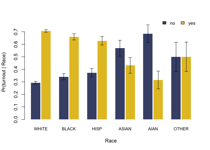

A more detailed introduction to the method and software package can be found on the Get Started page.