The US Census Bureau releases redistricting data (P.L. 94-171) following the decennial census. This article walks through the basics of reading that data and getting it into working form.
The P.L. 94-171 Legacy File
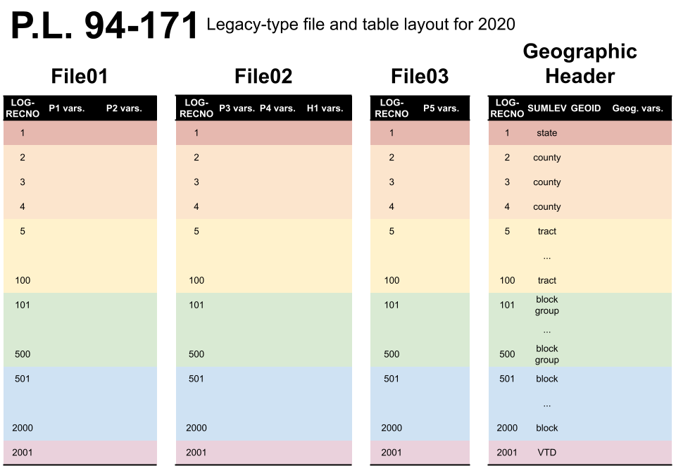
The redistricting data mandated by P.L. 94-171 is composed of six tables, five of population characteristics, and one of housing characteristics. In the legacy data format, these six tables (and dozens of levels of geography) are split into four files: File01, File02, File03, and the Geographic Header Record. Files 01–03 have the actual decennial census data for each table, while the geographic header has geographic identifiers (FIPS code, precinct IDs, etc.) and information (area, water, etc.).

These four files have the same rows, each of which is identified by a
LOGRECNO number. Combining the columns shared across the
four files yields the full P.L. 94-171 file
The basic unit of Census geography is the block; all other
geographies are constructed from them. But the P.L. 94-171 file is not
composed of blocks alone. The Census has already tabulated the six table
statistics across every possible level of geographies. To get
information for a single geography level—blocks, or counties, or school
districts—one needs only to subset to the rows which correspond to this
geographic level (coded in the SUMLEV column).
So the basic process for working with legacy P.L. 94-171 data is:
- Read in the four P.L. files (
pl_read(),pl_url()) - Combine the four files into one, and subset to the desired geography
level (
pl_subset(); geography level codes listed inpl_geog_levels) - Select the desired variables from the six included tables
(
pl_select_standard()) - Optionally, combine the processed data with the corresponding
tigrisshapefile.
The utility function pl_tidy_shp() combines all of these
steps into one function for most common use case of tabulating basic
redistricting information at the block level. This is demonstrated in the README
Using the PL94171 package
The four components of the P.L. 94-171 file should be downloaded into
their own directory. Here, we’ll use the example data included in the
package, from the 2018 end-to-end Census test in Providence County,
Rhode Island, and read it into our R session. In general, you can
provide a URL in place of a file path, and the package will read the
data from the URL. The pl_url() function will automatically
construct the URL to the data for a given state and year.
# `extdata/ri2018_2020Style.pl` is a directory with the four P.L. 94-171 files
path <- system.file("extdata/ri2018_2020Style.pl", package = "PL94171")
pl_raw <- pl_read(path)
# try `pl_read(pl_url("RI", 2010))`
This creates a large list where each individual P.L. 94-171 file
component is a separate entry in the list. If we look at the top of one
of these entries, we see the same structure as in the schematic above:
each redistricting variable is a column, the rows are indexed by
LOGRECNO, and various levels of aggregation are all
included as different sets of rows in the same table (notice the
countywide population counts in the first two rows).
head(pl_raw$`00003`)
#> # A tibble: 6 × 15
#>   FILEID STUSAB CHARITER CIFSN LOGRECNO P0050001 P0050002 P0050003 P0050004
#>   <chr>  <chr>  <chr>    <chr>    <int>    <int>    <int>    <int>    <int>
#> 1 PLST   RI     000      03           1    15766     7311     3266      261
#> 2 PLST   RI     000      03           2    15766     7311     3266      261
#> 3 PLST   RI     000      03          19      732        0        0        0
#> 4 PLST   RI     000      03          20        0        0        0        0
#> 5 PLST   RI     000      03          21        1        0        0        0
#> 6 PLST   RI     000      03          22        1        1        0        0
#> # ℹ 6 more variables: P0050005 <int>, P0050006 <int>, P0050007 <int>,
#> #   P0050008 <int>, P0050009 <int>, P0050010 <int>
To subset to a desired geography level, we must first identify the
corresponding SUMLEV code.
print(pl_geog_levels)
#> # A tibble: 85 × 2
#>    SUMLEV SUMLEV_description
#>    <chr>  <chr>
#>  1 040    State
#>  2 050    State-County
#>  3 060    State-County-County Subdivision
#>  4 067    State-County-County Subdivision-Subminor Civil Division
#>  5 140    State-County-Census Tract
#>  6 150    State-County-Census Tract-Block Group
#>  7 155    State-Place-County
#>  8 160    State-Place
#>  9 170    State-Consolidated City
#> 10 172    State-Consolidated City-Place within Consolidated City
#> # ℹ 75 more rows
Here, we’ll look at Census tracts, which are
SUMLEV=140.
We see that all four components have been combined into one large table, with data for each of the seven Census tracts in the example file recorded in a single row. To extract commonly-used variables from the 397 columns, we can run the following:
pl <- pl_select_standard(pl, clean_names = TRUE)
print(pl)
#> # A tibble: 7 × 24
#>   GEOID       state county row_id summary_level vtd     pop pop_hisp pop_white
#>   <chr>       <chr> <chr>   <int> <chr>         <chr> <int>    <int>     <int>
#> 1 44007000101 RI    007        19 140           NA     3970     1442      1445
#> 2 44007000102 RI    007        20 140           NA     4735     2555       815
#> 3 44007000200 RI    007        21 140           NA     5703     3766       570
#> 4 44007000300 RI    007        22 140           NA     6647     3827       754
#> 5 44007000400 RI    007        23 140           NA     3433     2130       142
#> 6 44007000500 RI    007        24 140           NA     2940     2249        39
#> 7 44007000600 RI    007        25 140           NA     1797      778       170
#> # ℹ 15 more variables: pop_black <int>, pop_aian <int>, pop_asian <int>,
#> #   pop_nhpi <int>, pop_other <int>, pop_two <int>, vap <int>, vap_hisp <int>,
#> #   vap_white <int>, vap_black <int>, vap_aian <int>, vap_asian <int>,
#> #   vap_nhpi <int>, vap_other <int>, vap_two <int>
Above, we set clean_names = TRUE, which is the default.
This creates a set of variables familiar to the redist
family of packages.
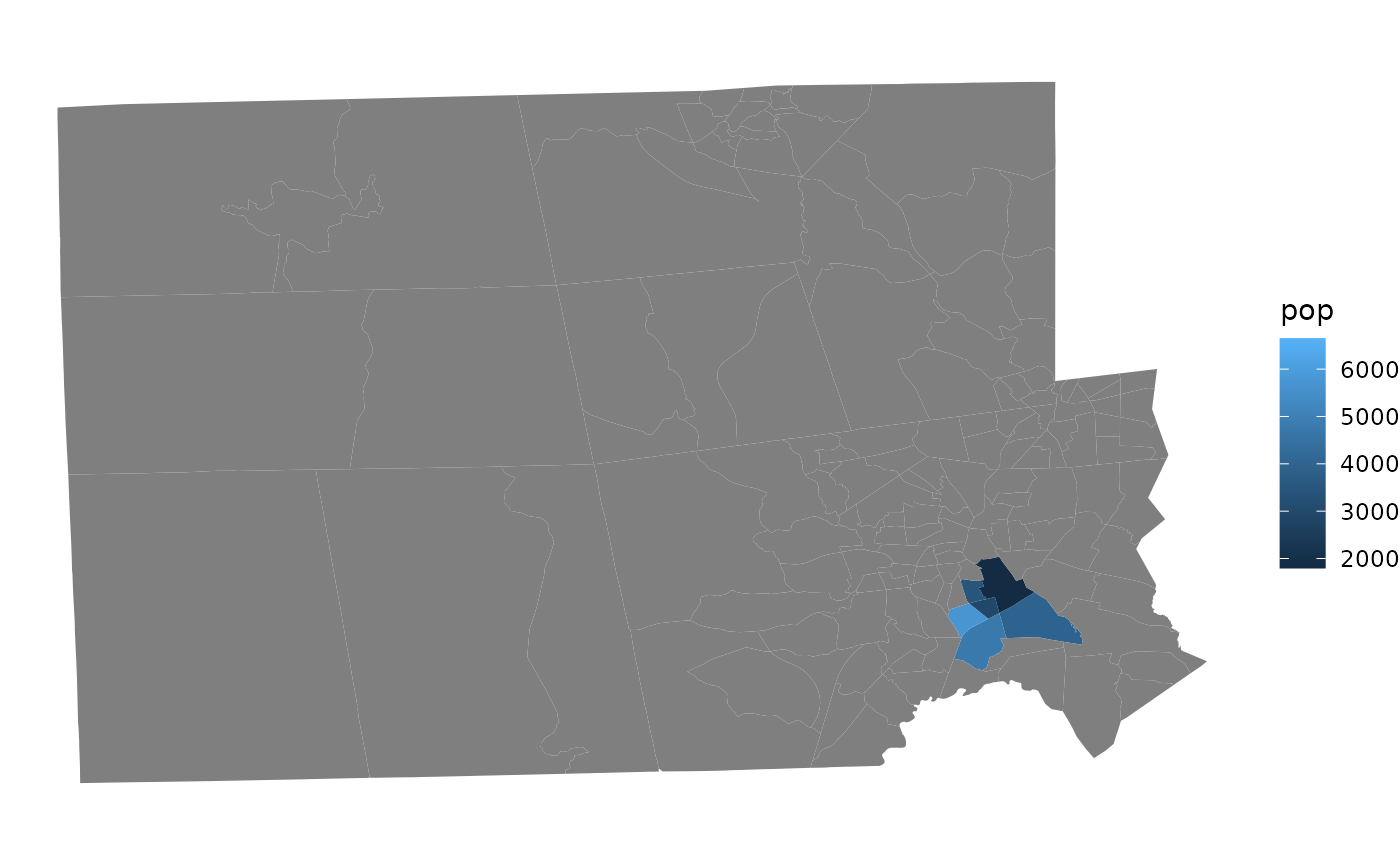
To combine these data with a shapefile, we must use the
tinytiger package. The GEOID column is shared
between the P.L. 94-171 data and the TIGER shapefiles from
tinytiger.
library(tinytiger)
library(sf)
library(dplyr)
library(ggplot2)

ri_tracts = tt_tracts("RI", county="Providence", year=2020)
#> Linking to GEOS 3.12.1, GDAL 3.8.4, PROJ 9.4.0; sf_use_s2() is TRUE
#>
#> Attaching package: 'dplyr'
#> The following objects are masked from 'package:stats':
#>
#> filter, lag
#> The following objects are masked from 'package:base':
#>
#> intersect, setdiff, setequal, unionThen we can join the shapes and data
full_join(pl, ri_tracts, by="GEOID") %>%
ggplot(aes(fill=pop, geometry=geometry)) +
    geom_sf(size=0) +
    theme_void()