ACS-Decennial-Block Harmonization

This vignette examines the accuracy of the ACS-Decennial-Block harmonization calculated by bl_harmonize_vars(). We start where the README leaves off.

library(blockpop)
library(dplyr)
library(stringr)
library(tidyr)

acs_d = bl_download_acs_vars("WA")
census_d = bl_download_2010_vars("WA")

block_d = bl_download_fcc("data-raw/fcc.csv") %>%
    bl_load_state("WA", .) %>%
    bl_est_2020() %>%
    bl_harmonize_vars(census_d, acs_d)
print(block_d)

Then we join summarize our block-level estimates at the block group level and join them to the ACS data to compare.

sum_d = block_d %>%
    select(-starts_with("vap_")) %>%
    mutate(bgroup = str_sub(block, 1, 12)) %>%
    select(-block, -state) %>%
    group_by(bgroup) %>%
    summarize(across(everything(), sum)) %>%
    rename_with(~ str_c("est_", .), .cols=starts_with("pop_")) %>%
    inner_join(rename_with(acs_d, ~ str_c("acs_", .), 
                           .cols=-bgroup), by="bgroup") %>%
    pivot_longer(c(starts_with("est_pop_"), starts_with("acs_pop_")),
                 names_to=c("source", "type", "race"),
                 names_sep="_", values_to="count") %>%
    select(-type) %>%
    pivot_wider(names_from=source, values_from=count) %>%
    mutate(est_pct = est/pop2020,
           acs_pct = acs/acs_pop)

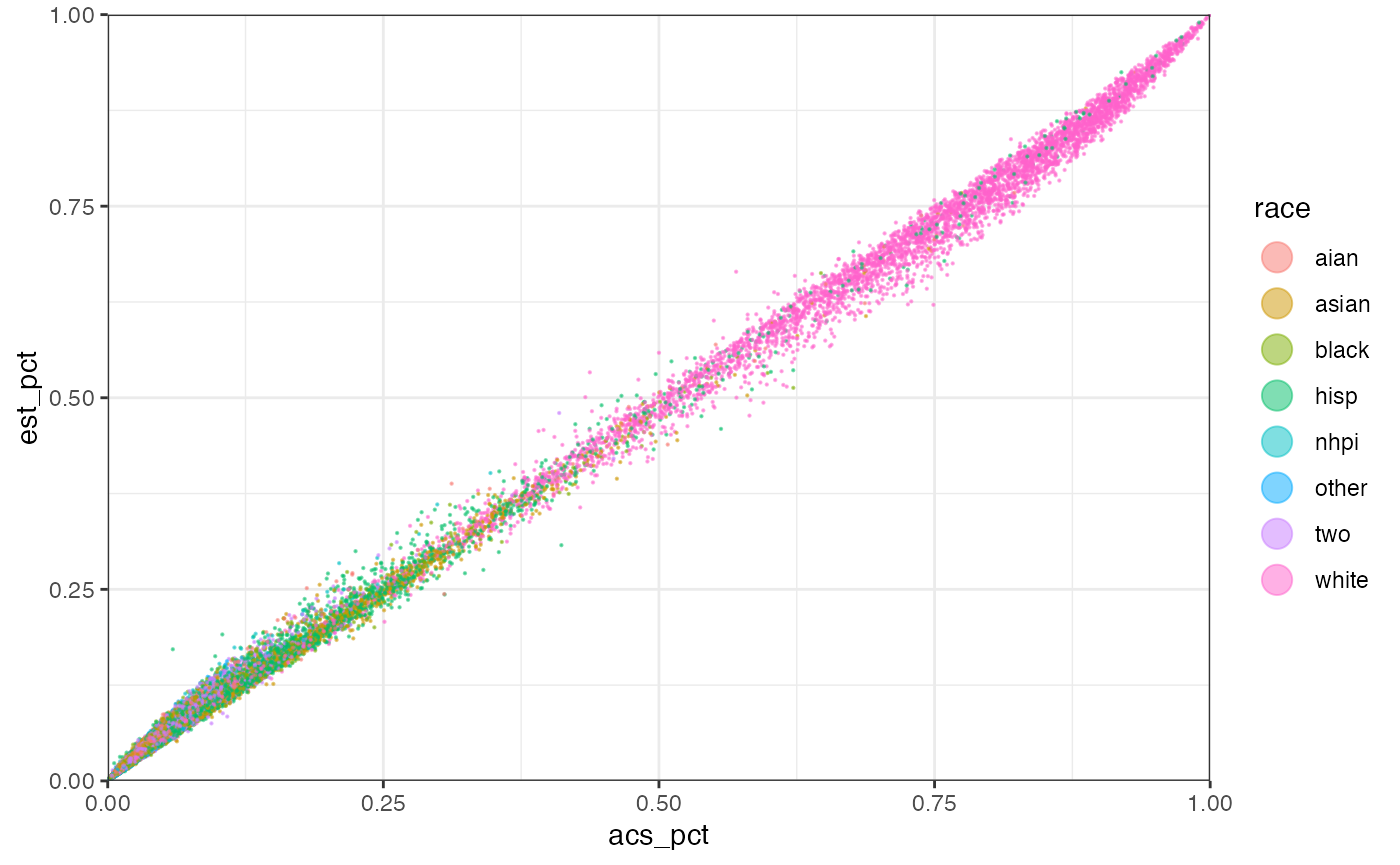
Plotting, we see excellent agreement between the ACS and estimated demographic percentages at the block group level. In fact, the Spearman correlation is in excess of 99.9%.

library(ggplot2)

ggplot(sum_d, aes(acs_pct, est_pct, color=race)) +
    geom_point(size=0.1, alpha=0.5) +
    coord_cartesian(expand=0) +
    guides(color=guide_legend(override.aes=list(size=5))) +
    theme_bw() 
#> Warning: Removed 96 rows containing missing values (geom_point).

This agreement occurs with 2020 block total population estimates exactly equal to the projections from bl_est_2020(), and using block-level demographic estimates that are as close as possible to the 2010 Census counts. This means much more accuracy and granularity than simple population-based disaggregation from block-group-level ACS data.