Analyzing aggregate data • seine

Ecological inference (EI) is the statistical problem of learning individual-level associations from aggregate-level data. EI commonly arises when two datasets are joined using a shared geographic identifier, and when individual data are not released for privacy reasons. To take some recent examples from the New York Times:

EI is also used in public health and epidemiology, and is widely applied in litigation under the federal Voting Rights Act of 1965 (VRA) to establish the presence of racially polarized voting.

Preparing data

As an example of an ecological analysis, we will use the elec_1968 data included in the package. The data contain county-level election returns from Southern states in the 1968 U.S. presidential election along with a number of covariates taken from the 1970 U.S. census. The counties here are the aggregation units; in other analyses, states, precincts, or cities might be the aggregation units.

library(seine)
data(elec_1968)

print(elec_1968)
#> # A tibble: 1,143 × 41
#>    fips  state  abbr  region division county    pop pop_city pop_urban pop_rural
#>    <chr> <chr>  <chr> <chr>  <chr>    <chr>   <dbl>    <dbl>     <dbl>     <dbl>
#>  1 01001 Alaba… AL    South  East So… Autau…  24460        0     0.536     0.464
#>  2 01003 Alaba… AL    South  East So… Baldw…  59382        0     0.266     0.734
#>  3 01005 Alaba… AL    South  East So… Barbo…  22543        0     0.404     0.596
#>  4 01007 Alaba… AL    South  East So… Bibb …  13812        0     0         1    
#>  5 01009 Alaba… AL    South  East So… Bloun…  26853        0     0.163     0.837
#>  6 01011 Alaba… AL    South  East So… Bullo…  11824        0     0.366     0.634
#>  7 01013 Alaba… AL    South  East So… Butle…  22007        0     0.365     0.635
#>  8 01015 Alaba… AL    South  East So… Calho… 103092        0     0.641     0.359
#>  9 01017 Alaba… AL    South  East So… Chamb…  36356        0     0.437     0.563
#> 10 01019 Alaba… AL    South  East So… Chero…  15606        0     0         1    
#> # ℹ 1,133 more rows
#> # ℹ 31 more variables: pop_white <dbl>, pop_black <dbl>, pop_aian <dbl>,
#> #   pop_asian <dbl>, pop_hisp <dbl>, vap <dbl>, vap_white <dbl>,
#> #   vap_black <dbl>, vap_other <dbl>, farm <dbl>, nonfarm <dbl>,
#> #   educ_elem <dbl>, educ_hsch <dbl>, educ_coll <dbl>, cvap <dbl>,
#> #   cvap_white <dbl>, cvap_black <dbl>, cvap_other <dbl>, inc_00_03k <dbl>,
#> #   inc_03_08k <dbl>, inc_08_25k <dbl>, inc_25_99k <dbl>, pres_dem_hum <dbl>, …

We are interested in estimating the individual-level association between race and presidential vote choice. The outcome variables are the proportion of votes cast for each candidate: pres_dem_hum, pres_rep_nix, pres_ind_wal, and pres_abs, where the latter are abstentions and ballots cast for other candidates. The predictor variables are the proportions of the voting-age population in each racial group: vap_white, vap_black, and vap_other. The data also contain a number of covariates, such as education and income, which we discuss below.

Ideally, these would be the proportion of each racial group within the population that actually cast a ballot for President. Since those proportions are unobserved, they would have to be estimated using a first stage of ecological inference with an outcome variable measuring turnout. Alternatively, one could include non-voters as another category of outcome variable, so that both outcome and predictor variables are proportions relative to the total voting-age population. For demonstration purposes, we will ignore this issue and proceed as if turnout were uniform across racial groups in every county.

These data have already been cleaned. Often, outcomes and predictors are measured as counts, or may have been rounded, so that they do not sum to exactly 1. seine provides the ei_proportions() function to assist in preprocessing. To see this in action, suppose we wanted to set up the turnout problem mentioned in the previous paragraph. The ei_proportions() function would let us create a new turnout proportion variable from our existing data.

elec_1968_turn = ei_proportions(elec_1968, turnout = pres_total, 
                                .total = vap, clamp = 0.01)

subset(elec_1968_turn, select = c(fips, state, county, turnout, vap, .other))
#> # A tibble: 1,143 × 6
#>    fips  state   county          turnout   vap .other
#>    <chr> <chr>   <chr>             <dbl> <dbl>  <dbl>
#>  1 01001 Alabama Autauga County    0.606 12744  0.394
#>  2 01003 Alabama Baldwin County    0.568 33012  0.432
#>  3 01005 Alabama Barbour County    0.645 12370  0.355
#>  4 01007 Alabama Bibb County       0.601  7575  0.399
#>  5 01009 Alabama Blount County     0.566 15856  0.434
#>  6 01011 Alabama Bullock County    0.721  6019  0.279
#>  7 01013 Alabama Butler County     0.593 12341  0.407
#>  8 01015 Alabama Calhoun County    0.484 55547  0.516
#>  9 01017 Alabama Chambers County   0.504 21117  0.496
#> 10 01019 Alabama Cherokee County   0.614  9215  0.386
#> # ℹ 1,133 more rows

The function normalizes pres_total by vap and stores the result in a column labeled turnout. It also stores the remaining proportion (i.e., the non-voters) in the .other column, by default. In this data, there is one county which had higher turnout than 1970 VAP. The clamp = 0.01 argument tells ei_proportions() to allow that kind of excess up to 1% of the total, and round those proportions down to 1. Any proportions in excess of 1.01 would throw an error. You can read about other functionality and customization of ei_proportions() in the function’s documentation.

Avoiding the ecological fallacy

The core challenge of ecological inference is that only marginal proportions are observed (racial groups, candidate vote shares), but we are interested in joint data (candidate vote shares within each racial group). The key to overcoming this challenge is assuming some kind of homogeneity across aggregation units. Enough homogeneity means that information can be shared across aggregation units to estimate the missing joint proportions.

More precisely, a researcher needs to believe that coarsening at random (CAR) holds in order to conduct EI. Coarsening at random means that unobserved joint data of interest are mean-independent of the predictors and the number of people in each aggregation unit, given covariates.¹

In these data, CAR means that once we know a set of covariate values for a county, such as its education and age, learning about the racial composition of the county does not change our beliefs about the candidate preference within each racial group or the total turnout.

For example, take the three counties shown below, which have been selected by a clustering algorithm to be similar on the observed covariates: urbanity, agriculture, education, and income.

state	county	farm	educ_elem	educ_hsch	educ_coll	inc_00_03k	inc_03_08k	inc_08_25k	inc_25_99k
Virginia	Charles City County	0.0409	0.5401	0.3669	0.0930	0.1778	0.4486	0.3570	0.0166
Virginia	Greene County	0.0737	0.5827	0.3517	0.0656	0.1736	0.3832	0.4368	0.0064
Virginia	Louisa County	0.0620	0.5300	0.3964	0.0736	0.1823	0.4200	0.3814	0.0163

CAR means that the preference for, e.g., George Wallace among White voters in these counties is roughly the same and is unrelated to the fact that the demographics are quite different between the counties:

state	county	vap_white	vap_black	vap_other	pres_total
Virginia	Charles City County	0.2138	0.7000	0.0862	1960
Virginia	Greene County	0.9073	0.0917	0.0010	1549
Virginia	Louisa County	0.6669	0.3318	0.0014	3964

If we believed that in the majority-Black Charles City County, racial resentment might increase the preference for Wallace compared to the heavily majority-White Greene County, then CAR would be violated.

For now, we will proceed under the CAR assumption, though there are serious reasons to doubt its applicability in these data. Later, we’ll discuss how to conduct a sensitivity analysis to evaluate how possible violations might affect our conclusions.

Ecological estimation

Once we’ve evaluated the CAR assumption, we can proceed with estimation. seine implements double/debiased machine learning (DML), which means we fit two models before combining them for a final estimate:

A regression model of the outcome variables on the predictor variables and covariates
A Riesz representer model, which yields a special set of “weights” that can be used in estimation.

By carefully combining the fitted regression and Riesz representer, we can reduce the sensitivity to biases in each component.

Setup

seine provides both a formula interface and a tidy interface through a new ei_spec() object. We recommend the ei_spec() approach for most analyses, since it dovetails well with the other estimation and sensitivity functions. We will demonstrate both approaches here, however.

To create an EI specification, we call ei_spec() and use tidyselect syntax to specify the outcome, predictors, covariates, and the column with the total number of people in each aggregation unit.

spec = ei_spec(
    elec_1968, 
    predictors = vap_white:vap_other,
    outcome = pres_dem_hum:pres_abs, 
    total = pres_total,
    covariates = c(state, pop_city:pop_rural, farm:educ_coll, 
                   inc_00_03k:inc_25_99k)
)

print(spec)
#> EI Specification
#> • Predictors: `vap_white`, `vap_black`, and `vap_other`
#> • Outcome: `pres_dem_hum`, `pres_rep_nix`, `pres_ind_wal`, and `pres_abs`
#> • Covariates: `state`, `pop_city`, `pop_urban`, `pop_rural`, `farm`, `nonfarm`, `educ_elem`, `educ_hsch`, `educ_coll`, `inc_00_03k`, `inc_03_08k`, `inc_08_25k`, and `inc_25_99k`
#> # A tibble: 1,143 × 20
#>   vap_white vap_black vap_other pres_dem_hum pres_rep_nix pres_ind_wal pres_abs
#>       <dbl>     <dbl>     <dbl>        <dbl>        <dbl>        <dbl>    <dbl>
#> 1     0.761    0.237   0.00173        0.199        0.0773        0.711  0.0122 
#> 2     0.860    0.137   0.00306        0.105        0.115         0.764  0.0161 
#> 3     0.610    0.389   0.000808       0.242        0.0489        0.687  0.0218 
#> 4     0.783    0.216   0.00106        0.141        0.0571        0.799  0.00290
#> 5     0.981    0.0181  0.000757       0.0375       0.222         0.727  0.0134 
#> # ℹ 1,138 more rows
#> # ℹ 13 more variables: state <chr>, pop_city <dbl>, pop_urban <dbl>,
#> #   pop_rural <dbl>, farm <dbl>, nonfarm <dbl>, educ_elem <dbl>,
#> #   educ_hsch <dbl>, educ_coll <dbl>, inc_00_03k <dbl>, inc_03_08k <dbl>,
#> #   inc_08_25k <dbl>, inc_25_99k <dbl>

An ei_spec object is just a data frame with some additional metadata about these variables.

Fitting the regression

Any machine learning method can be used to fit the regression model. However, due to the aggregation process that led to our data, there is certain structure in the regression function that can be leveraged for improved estimation. We recommend using ei_ridge() to fit the regression model, because it will automatically use this structure, and automatically determine the ridge penalty using a closed-form expression for the leave-one-out errors. To make the regression nonparametric, basis expansions such as kernel functions, polynomials, or splines can be used. The bases package and the built-in splines package provide functions that carry out these expansions and can be used inside model formulas.

Using the tidy interface, fitting the regression is as simple as calling ei_ridge() on the ei_spec object:

m = ei_ridge(spec)

print(m)
#> An ecological inference model with 4 outcomes, 3 groups, and 1143 observations
#> Fit with penalty = 0.0432704

We can see that ei_ridge() has automatically selected a small ridge penalty. By default, all covariates are centered and scaled to have unit variance. This is generally appropriate when penalizing all coefficients equally, as is done by ei_ridge(). But in some cases it may not be appropriate, and this behavior can be suppressed by providing scale = FALSE.

Alternatively, we could use the formula interface, which would also let us specify our own interaction terms; here, we interact state with all other variables. Formulas in seine require the user separate the predictors and covariates by a vertical bar.

m_form = ei_ridge(
    cbind(pres_dem_hum, pres_rep_nix, pres_ind_wal, pres_abs) ~ 
        vap_white + vap_black + vap_other | 
        state * (pop_urban + pop_rural + farm + educ_hsch + educ_coll +
                     inc_03_08k + inc_08_25k + inc_25_99k),
    data = elec_1968, total = pres_total
)

print(m_form)
#> An ecological inference model with 4 outcomes, 3 groups, and 1143 observations
#> Fit with penalty = 5.22561

The summary() method of fitted regression objects shows summary statistics for fitted values, which can help diagnose misspecification, and shows the \(R^2\) values for each outcome variable. Here, racial demographics and covariates explain a substantial amount of the total variation in vote shares. The fitted values are almost all between 0 and 1, but the presence of some negative predictions indicates there is at least some model misspecification.

summary(m)
#> Fitted values:
#>   pres_dem_hum      pres_rep_nix      pres_ind_wal         pres_abs         
#>  Min.   :0.01289   Min.   :-0.0296   Min.   :-0.01479   Min.   :-0.0012395  
#>  1st Qu.:0.23672   1st Qu.: 0.1911   1st Qu.: 0.26210   1st Qu.:-0.0001323  
#>  Median :0.29178   Median : 0.3110   Median : 0.37332   Median : 0.0001229  
#>  Mean   :0.30163   Mean   : 0.2970   Mean   : 0.40004   Mean   : 0.0013323  
#>  3rd Qu.:0.37902   3rd Qu.: 0.3890   3rd Qu.: 0.53561   3rd Qu.: 0.0005280  
#>  Max.   :0.70426   Max.   : 0.6481   Max.   : 0.84246   Max.   : 0.0142096  
#> 
#> R-squared by outcome:
#> pres_dem_hum pres_rep_nix pres_ind_wal     pres_abs 
#>    0.6880171    0.7165231    0.8114222    0.5441581

Fitting the Riesz representer

The Riesz representer is less familiar, but no less easy to fit. Using the tidy interface, we simply pass the ei_spec object to ei_riesz(). Unlike ei_ridge(), ei_riesz() requires a penalty to be specified. A good default is to use the same penalty as was used in the regression.

rr = ei_riesz(spec, penalty = m$penalty)

We could also use the formula interface. It is critical to provide exactly the same formula and data to both ei_ridge() and ei_riesz() (though the Riesz representer does not use the outcome variable); the tidy interface obviates the need to worry about this.

rr_form = ei_riesz(
    ~ vap_white + vap_black + vap_other | 
        state * (pop_urban + pop_rural + farm + educ_hsch + educ_coll +
                     inc_03_08k + inc_08_25k + inc_25_99k),
    data = elec_1968, total = pres_total, penalty = m_form$penalty
)

As with the regression model, the summary() function provides useful information for evaluating the Riesz representer.

summary(rr)
#> Second moment of representer:
#>    vap_white    vap_black    vap_other 
#>     15.01799    228.39141 103472.19420 
#> 
#> Second moment of representer (leave-one-out):
#>    vap_white    vap_black    vap_other 
#>     17.25841    257.75390 144881.23787

Large second moments of the Riesz representer are indicative of a more difficult EI problem, likely due to limited variation in the predictor, given covariates. Here we see that there is very little information for the other group, and the representer is highly variable. Comparing the in-sample and leave-one-out second moments can also help identify cases of possible overfitting, where a higher penalty may be useful.

DML for ecological estimates

With the regression function and Riesz representer now fitted, we are ready to combine them to estimate our quantities of interest: vote choice by race. This is accomplished with the ei_est() function, which takes in both fitted models and the original ei_spec object, and returns a tidy data frame of estimates. The conf_level argument is optional and produces confidence intervals of the specified width from the asymptotic Normal approximation.

est = ei_est(m, rr, spec, conf_level = 0.95)
print(est)
#> # A tibble: 12 × 6
#>    predictor outcome      estimate std.error  conf.low conf.high
#>    <chr>     <chr>           <dbl>     <dbl>     <dbl>     <dbl>
#>  1 vap_white pres_dem_hum  0.225    0.0241    0.178      0.273  
#>  2 vap_black pres_dem_hum  0.584    0.0601    0.467      0.702  
#>  3 vap_other pres_dem_hum  2.92     0.744     1.47       4.38   
#>  4 vap_white pres_rep_nix  0.435    0.0365    0.363      0.506  
#>  5 vap_black pres_rep_nix -0.0242   0.0367   -0.0962     0.0477 
#>  6 vap_other pres_rep_nix -4.75     0.991    -6.69      -2.81   
#>  7 vap_white pres_ind_wal  0.339    0.0197    0.300      0.377  
#>  8 vap_black pres_ind_wal  0.437    0.0436    0.351      0.522  
#>  9 vap_other pres_ind_wal  2.84     0.840     1.20       4.49   
#> 10 vap_white pres_abs      0.00145  0.000384  0.000692   0.00220
#> 11 vap_black pres_abs      0.00314  0.00111   0.000957   0.00532
#> 12 vap_other pres_abs     -0.0186   0.0265   -0.0706     0.0334

The same call works with the formula interface.

est_form = ei_est(m_form, rr_form, elec_1968)

Occasionally, it is helpful to examine the estimates in a different format. The as.matrix() method works on ei_est objects and can be used on any column of the object, such as the estimate or standard error. The full (asymptotic) covariance matrix of all estimates is also accessible via vcov().

as.matrix(est)
#>            outcome
#> predictor   pres_dem_hum pres_rep_nix pres_ind_wal     pres_abs
#>   vap_white    0.2253004   0.43469163    0.3385627  0.001445307
#>   vap_black    0.5844989  -0.02422778    0.4365898  0.003139145
#>   vap_other    2.9232285  -4.74841187    2.8437828 -0.018599469

as.matrix(est, which = "conf.low")
#>            outcome
#> predictor   pres_dem_hum pres_rep_nix pres_ind_wal      pres_abs
#>   vap_white    0.1780894   0.36318338    0.2998869  0.0006917330
#>   vap_black    0.4666862  -0.09617439    0.3512261  0.0009571476
#>   vap_other    1.4658425  -6.69044611    1.1971298 -0.0705544420

Sometimes, estimates within a set of geographies are of interest. The subset= argument to ei_est() allows for producing estimates in these smaller areas.

as.matrix(ei_est(m, rr, spec, subset = (state == "Mississippi")))
#>            outcome
#> predictor   pres_dem_hum pres_rep_nix pres_ind_wal     pres_abs
#>   vap_white  0.002209141   0.19864269    0.7995612 -0.000413015
#>   vap_black  0.738043281   0.01895925    0.2413356  0.001661887
#>   vap_other  1.405217200  -2.76253073    2.3609276 -0.003614053

Finally, ei_est() actually also works with a regression model alone, or a Riesz representer alone. However, these estimates are not debiased, and may have higher error. They generally have improperly calibrated confidence intervals.

# Not recommended
est_m = ei_est(regr = m, data = spec)
est_rr = ei_est(riesz = rr, data = spec)

sd(est_m$estimate - est_rr$estimate) # estimates (here) are close
#> [1] 0.005069123
sd(est_m$std.error - est_rr$std.error) # standard errors are very different
#> [1] 1.331431

Sensitivity analysis

The entire analysis so far has rested on the critical CAR assumption. In practice, no such independence assumption ever holds exactly. Thus, it is important to evaluate how sensitive the results are to violations of that identifying assumption.

seine provides a number of tools to do this. All are based on a nonparametric sensitivity framework developed by Chernozhukov et al. (2024). This framework considers the relationship between an unobserved confounding variable and the outcome and predictors, measured in terms of certain partial \(R^2\) values. Essentially, the stronger the relationship, the more confounding is present and the more biased the original estimates are.

The ei_sens() function provides a simple interface to this framework. Users provide values for sensitivity parameters, and a bound on the absolute bias is returned. In the following example, we investigate the effect of an omitted confounder that explains 50% of the residual variation in the outcome and 20% of the variation in the Riesz representer, compared to the true representer.

ei_sens(est, c_outcome = 0.5, c_predictor = 0.2)
#> # A tibble: 12 × 9
#>    predictor outcome estimate std.error conf.low conf.high c_outcome c_predictor
#>    <chr>     <chr>      <dbl>     <dbl>    <dbl>     <dbl>     <dbl>       <dbl>
#>  1 vap_white pres_d…  0.225    0.0241    7.52e-2   0.375         0.5         0.2
#>  2 vap_black pres_d…  0.584    0.0601    9.78e-2   1.07          0.5         0.2
#>  3 vap_other pres_d…  2.92     0.744    -9.98e+0  15.8           0.5         0.2
#>  4 vap_white pres_r…  0.435    0.0365    2.44e-1   0.626         0.5         0.2
#>  5 vap_black pres_r… -0.0242   0.0367   -5.24e-1   0.476         0.5         0.2
#>  6 vap_other pres_r… -4.75     0.991    -2.00e+1  10.5           0.5         0.2
#>  7 vap_white pres_i…  0.339    0.0197    1.72e-1   0.505         0.5         0.2
#>  8 vap_black pres_i…  0.437    0.0436   -1.06e-1   0.979         0.5         0.2
#>  9 vap_other pres_i…  2.84     0.840    -1.30e+1  18.7           0.5         0.2
#> 10 vap_white pres_a…  0.00145  0.000384 -3.79e-3   0.00668       0.5         0.2
#> 11 vap_black pres_a…  0.00314  0.00111  -1.51e-2   0.0214        0.5         0.2
#> 12 vap_other pres_a… -0.0186   0.0265   -5.69e-1   0.532         0.5         0.2
#> # ℹ 1 more variable: bias_bound <dbl>

We can also work backwards and ask what one of the sensitivity parameters would have to be in order to produce a certain amount of bias. For example, if we assumed a worst-case scenario where the confounder explains the entire outcome (c_outcome = 1), we can ask how strongly that confounder would need to be related to the Riesz representer to produce a bias of up to 5pp.

ei_sens(est, c_outcome = 1, bias_bound = 0.05)
#> # A tibble: 12 × 9
#>    predictor outcome estimate std.error conf.low conf.high c_outcome c_predictor
#>    <chr>     <chr>      <dbl>     <dbl>    <dbl>     <dbl>     <dbl>       <dbl>
#>  1 vap_white pres_d…  0.225    0.0241     0.128     0.323          1  0.0287    
#>  2 vap_black pres_d…  0.584    0.0601     0.417     0.752          1  0.00229   
#>  3 vap_other pres_d…  2.92     0.744      1.42      4.43           1  0.00000239
#>  4 vap_white pres_r…  0.435    0.0365     0.313     0.556          1  0.0214    
#>  5 vap_black pres_r… -0.0242   0.0367    -0.146     0.0977         1  0.00170   
#>  6 vap_other pres_r… -4.75     0.991     -6.74     -2.76           1  0.00000177
#>  7 vap_white pres_i…  0.339    0.0197     0.250     0.427          1  0.0189    
#>  8 vap_black pres_i…  0.437    0.0436     0.301     0.572          1  0.00149   
#>  9 vap_other pres_i…  2.84     0.840      1.15      4.54           1  0.00000155
#> 10 vap_white pres_a…  0.00145  0.000384  -0.0493    0.0522         1  0.940     
#> 11 vap_black pres_a…  0.00314  0.00111   -0.0490    0.0553         1  0.547     
#> 12 vap_other pres_a… -0.0186   0.0265    -0.121     0.0834         1  0.00126   
#> # ℹ 1 more variable: bias_bound <dbl>

For most predictors and outcomes, the answer is not very much!

The c_outcome parameter is relatively easy to understand, but c_predictor is more difficult to interpret (though see the methodology paper for more discussion). To help understand plausible values of these parameters, we can conduct a benchmarking analysis that treats each of our observed covariates in turn as a hypothetical unobserved confounder, and then calculates the values of the sensitivity parameters in that instance. Because of the amount of automated inference behind the scenes, this analysis only works using the tidy estimation framework.

bench = ei_bench(spec)

subset(bench, predictor == "white" & outcome == "dem_hum")
#> # A tibble: 0 × 7
#> # ℹ 7 variables: covariate <chr>, predictor <chr>, outcome <chr>,
#> #   c_outcome <dbl>, c_predictor <dbl>, confounding <dbl>, est_chg <dbl>

The table above shows the benchmark values for each covariate for the White preference for Humphrey estimand. The confounding column is an additional component of the sensitivity analysis that is discussed in the paper; the default value is 1, which is a conservative worst-case bound. The benchmark values here show that state is far and away the strongest observed confounder, whose inclusion changes the estimate by 6.5pp. If the unobserved confounders were as strong as state, we might expect a significant amount of bias, as we will see next.

Rather than perform this sensitivity analysis on a single set of sensitivity parameters, we can run it across all combinations of parameter values, and visualize the results on a bias contour plot. We can further overlay the benchmarking values to help interpret the results.

sens = ei_sens(est) # the default evaluates on a grid of parameters
plot(sens, bench = bench)

Bias contour plot for the White preference for Humphrey

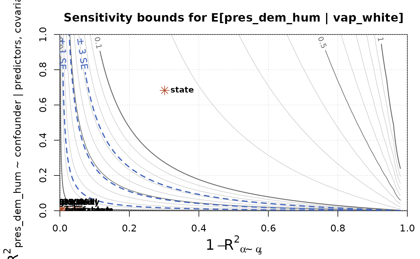
The contour lines indicate how much bias could result from an unobserved confounder with the specified sensitivity parameters. The blue dashed contours correspond to bias of 1, 2, and 3 standard errors. This is a helpful value to compare against, because bias of that size corresponds to a predictable drop in coverage rates of confidence intervals. For example, bias of 1 standard error means that a confidence interval with 95% nominal coverage will actually have coverage of only around 80%.

The red asterisks indicate the benchmark values for each covariate. Most are clustered in the lower-left corner and can’t be distinguished. In contrast, the benchmark for state shows that an unobserved confounder of that strength could lead to bias of around 15pp, which is substantial compared to the estimate itself, which is 22.5pp.

Finally, it can be helpful to summarize the sensitivity analysis by a single number. The ei_sens_rv() function calculates the robustness value, which measures the minimum strength of an unobserved confounder that would lead to a bias of a given amount. Here, we might consider a bias of one standard error to be problematic, due to its implications for the coverage of our confidence intervals.

ei_sens_rv(est, bias_bound = 1 * std.error)
#> # A tibble: 12 × 7
#>    predictor outcome      estimate std.error  conf.low conf.high     rv
#>    <chr>     <chr>           <dbl>     <dbl>     <dbl>     <dbl>  <dbl>
#>  1 vap_white pres_dem_hum  0.225    0.0241    0.178      0.273   0.0794
#>  2 vap_black pres_dem_hum  0.584    0.0601    0.467      0.702   0.0560
#>  3 vap_other pres_dem_hum  2.92     0.744     1.47       4.38    0.0227
#>  4 vap_white pres_rep_nix  0.435    0.0365    0.363      0.506   0.102 
#>  5 vap_black pres_rep_nix -0.0242   0.0367   -0.0962     0.0477  0.0299
#>  6 vap_other pres_rep_nix -4.75     0.991    -6.69      -2.81    0.0260
#>  7 vap_white pres_ind_wal  0.339    0.0197    0.300      0.377   0.0532
#>  8 vap_black pres_ind_wal  0.437    0.0436    0.351      0.522   0.0331
#>  9 vap_other pres_ind_wal  2.84     0.840     1.20       4.49    0.0207
#> 10 vap_white pres_abs      0.00145  0.000384  0.000692   0.00220 0.0299
#> 11 vap_black pres_abs      0.00314  0.00111   0.000957   0.00532 0.0242
#> 12 vap_other pres_abs     -0.0186   0.0265   -0.0706     0.0334  0.0186

All of the robustness values (one for each predictor/outcome combination) are relatively small, indicating low robustness (high sensitivity). In particular, they are all far smaller than the amount of confounding benchmarked by the observed state variable.

Alternatively, we might be interested in bias that would be sufficient to eliminate any evidence of racially polarized voting—i.e., to equalize the vote shares across racial groups. For clarity, we’ll show this analysis for just the Humphrey vote.

hum_avg = weighted.mean(elec_1968$pres_dem_hum, elec_1968$pres_total)
est_hum = subset(est, outcome == "dem_hum")
ei_sens_rv(est_hum, bias_bound = estimate - hum_avg)
#> # A tibble: 0 × 7
#> # ℹ 7 variables: predictor <chr>, outcome <chr>, estimate <dbl>,
#> #   std.error <dbl>, conf.low <dbl>, conf.high <dbl>, rv <dbl>

We see that it would take a larger amount of confounding, compared to the previous analysis, to eliminate evidence of racially polarized voting for Humprhey.

As with any single-number summary, it is important to consider sensitivity beyond the single value, by using the contour plot and the benchmarking analysis.

References

McCartan, C. and Kuriwaki, S. (2025+). Estimation of conditional means from aggregate data. Working paper.

Chernozhukov, V., Cinelli, C., Newey, W., Sharma, A., & Syrgkanis, V. (2024). Long story short: Omitted variable bias in causal machine learning (No. w30302). National Bureau of Economic Research.